Toy Examples with Code

Preamble

import numpy as np
from pysr import *

1. Simple search

Here's a simple example where we find the expression 2 cos(x3) + x0^2 - 2.

X = 2 * np.random.randn(100, 5)
y = 2 * np.cos(X[:, 3]) + X[:, 0] ** 2 - 2
model = PySRRegressor(binary_operators=["+", "-", "*", "/"])
model.fit(X, y)
print(model)

2. Custom operator

Here, we define a custom operator and use it to find an expression:

X = 2 * np.random.randn(100, 5)
y = 1 / X[:, 0]
model = PySRRegressor(
    binary_operators=["+", "*"],
    unary_operators=["inv(x) = 1/x"],
    extra_sympy_mappings={"inv": lambda x: 1/x},
)
model.fit(X, y)
print(model)

3. Multiple outputs

Here, we do the same thing, but with multiple expressions at once, each requiring a different feature.

X = 2 * np.random.randn(100, 5)
y = 1 / X[:, [0, 1, 2]]
model = PySRRegressor(
    binary_operators=["+", "*"],
    unary_operators=["inv(x) = 1/x"],
    extra_sympy_mappings={"inv": lambda x: 1/x},
)
model.fit(X, y)

4. Plotting an expression

For now, let's consider the expressions for output 0. We can see the LaTeX version of this with:

model.latex()[0]

or output 1 with model.latex()[1].

Let's plot the prediction against the truth:

from matplotlib import pyplot as plt
plt.scatter(y[:, 0], model.predict(X)[:, 0])
plt.xlabel('Truth')
plt.ylabel('Prediction')
plt.show()

Which gives us:

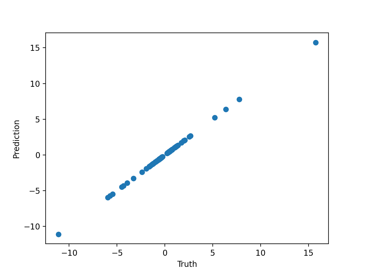
We may also plot the output of a particular expression by passing the index of the expression to predict (or sympy or latex as well)

5. Feature selection

PySR and evolution-based symbolic regression in general performs very poorly when the number of features is large. Even, say, 10 features might be too much for a typical equation search.

If you are dealing with high-dimensional data with a particular type of structure, you might consider using deep learning to break the problem into smaller "chunks" which can then be solved by PySR, as explained in the paper 2006.11287.

For tabular datasets, this is a bit trickier. Luckily, PySR has a built-in feature selection mechanism. Simply declare the parameter select_k_features=5, for selecting the most important 5 features.

Here is an example. Let's say we have 30 input features and 300 data points, but only 2 of those features are actually used:

X = np.random.randn(300, 30)
y = X[:, 3]**2 - X[:, 19]**2 + 1.5

Let's create a model with the feature selection argument set up:

model = PySRRegressor(
    binary_operators=["+", "-", "*", "/"],
    unary_operators=["exp"],
    select_k_features=5,
)

Now let's fit this:

model.fit(X, y)

Before the Julia backend is launched, you can see the string:

Using features ['x3', 'x5', 'x7', 'x19', 'x21']

which indicates that the feature selection (powered by a gradient-boosting tree) has successfully selected the relevant two features.

This fit should find the solution quickly, whereas with the huge number of features, it would have struggled.

This simple preprocessing step is enough to simplify our tabular dataset, but again, for more structured datasets, you should try the deep learning approach mentioned above.

6. Denoising

Many datasets, especially in the observational sciences, contain intrinsic noise. PySR is noise robust itself, as it is simply optimizing a loss function, but there are still some additional steps you can take to reduce the effect of noise.

One thing you could do, which we won't detail here, is to create a custom log-likelihood given some assumed noise model. By passing weights to the fit function, and defining a custom loss function such as elementwise_loss="myloss(x, y, w) = w * (x - y)^2", you can define any sort of log-likelihood you wish. (However, note that it must be bounded at zero)

However, the simplest thing to do is preprocessing, just like for feature selection. To do this, set the parameter denoise=True. This will fit a Gaussian process (containing a white noise kernel) to the input dataset, and predict new targets (which are assumed to be denoised) from that Gaussian process.

For example:

X = np.random.randn(100, 5)
noise = np.random.randn(100) * 0.1
y = np.exp(X[:, 0]) + X[:, 1] + X[:, 2] + noise

Let's create and fit a model with the denoising argument set up:

model = PySRRegressor(
    binary_operators=["+", "-", "*", "/"],
    unary_operators=["exp"],
    denoise=True,
)
model.fit(X, y)
print(model)

If all goes well, you should find that it predicts the correct input equation, without the noise term!

7. Julia packages and types

PySR uses SymbolicRegression.jl as its search backend. This is a pure Julia package, and so can interface easily with any other Julia package. For some tasks, it may be necessary to load such a package.

For example, let's say we wish to discovery the following relationship:

$$y=p_{3x+1}-5,$$

where $p_i$ is the $i$th prime number, and $x$ is the input feature.

Let's see if we can discover this using the Primes.jl package.

First, let's get the Julia backend:

from pysr import jl

jl stores the Julia runtime.

Now, let's run some Julia code to add the Primes.jl package to the PySR environment:

jl.seval("""
import Pkg
Pkg.add("Primes")
""")

This imports the Julia package manager, and uses it to install Primes.jl. Now let's import Primes.jl:

jl.seval("import Primes")

Now, we define a custom operator:

jl.seval("""
function p(i::T) where T
    if (0.5 < i < 1000)
        return T(Primes.prime(round(Int, i)))
    else
        return T(NaN)
    end
end
""")

We have created a a function p, which takes an arbitrary number as input. p first checks whether the input is between 0.5 and 1000. If out-of-bounds, it returns NaN. If in-bounds, it rounds it to the nearest integer, compures the corresponding prime number, and then converts it to the same type as input.

Next, let's generate a list of primes for our test dataset. Since we are using juliacall, we can just call p directly to do this:

primes = {i: jl.p(i*1.0) for i in range(1, 999)}

Next, let's use this list of primes to create a dataset of $x,y$ pairs:

import numpy as np

X = np.random.randint(0, 100, 100)[:, None]
y = [primes[3*X[i, 0] + 1] - 5 + np.random.randn()*0.001 for i in range(100)]

Note that we have also added a tiny bit of noise to the dataset.

Finally, let's create a PySR model, and pass the custom operator. We also need to define the sympy equivalent, which we can leave as a placeholder for now:

from pysr import PySRRegressor
import sympy

class sympy_p(sympy.Function):
    pass

model = PySRRegressor(
    binary_operators=["+", "-", "*", "/"],
    unary_operators=["p"],
    niterations=100,
    extra_sympy_mappings={"p": sympy_p}
)

We are all set to go! Let's see if we can find the true relation:

model.fit(X, y)

if all works out, you should be able to see the true relation (note that the constant offset might not be exactly 1, since it is allowed to round to the nearest integer). You can get the sympy version of the best equation with:

model.sympy()

8. Complex numbers

PySR can also search for complex-valued expressions. Simply pass data with a complex datatype (e.g., np.complex128), and PySR will automatically search for complex-valued expressions:

import numpy as np

X = np.random.randn(100, 1) + 1j * np.random.randn(100, 1)
y = (1 + 2j) * np.cos(X[:, 0] * (0.5 - 0.2j))

model = PySRRegressor(
    binary_operators=["+", "-", "*"], unary_operators=["cos"], niterations=100,
)

model.fit(X, y)

You can see that all of the learned constants are now complex numbers. We can get the sympy version of the best equation with:

model.sympy()

We can also make predictions normally, by passing complex data:

model.predict(X, -1)

to make predictions with the most accurate expression.

9. Custom objectives

Use loss_function when scoring needs the expression tree, symbolic manipulation, or auxiliary data from the dataset. Use loss_function_expression when it needs the complete expression object rather than its underlying tree. Both accept Julia source defining one of these signatures:

objective(tree_or_expression, dataset, options)
objective(tree_or_expression, dataset, options, idx=nothing)

With automatic batching, a three-argument objective receives a dataset already restricted to the active batch. A four-argument objective receives the full dataset and the selected row indices. This can be useful when needing to do custom batching operations.

The following batching-aware mean squared error is equivalent to the default objective for an unweighted scalar dataset:

objective = """
function mse_objective(tree, dataset::Dataset{T,L}, options, idx=nothing)::L where {T,L}
    X = idx === nothing ? dataset.X : dataset.X[:, idx]
    y = idx === nothing ? dataset.y : dataset.y[idx]
    prediction, complete = eval_tree_array(tree, X, options)
    complete || return L(Inf)
    return sum(abs2, prediction .- y) / length(y)
end
"""

model = PySRRegressor(
    loss_function=objective,
    binary_operators=["+", "-", "*", "/"],
)

Always check the completion flag returned by eval_tree_array; an incomplete evaluation must receive an infinite or suitably large loss. Return the dataset's loss type L, which needs to be real even when the data type T is complex.

A full objective can also reinterpret the tree. This example treats the two children of every binary root as a rational function $P(X)/Q(X)$:

objective = """
function rational_objective(tree, dataset::Dataset{T,L}, options, idx=nothing)::L where {T,L}
    tree.degree == 2 || return L(Inf)
    X = idx === nothing ? dataset.X : dataset.X[:, idx]
    y = idx === nothing ? dataset.y : dataset.y[idx]

    numerator = SymbolicRegression.InterfaceDynamicExpressionsModule.DE.get_child(tree, 1)
    denominator = SymbolicRegression.InterfaceDynamicExpressionsModule.DE.get_child(tree, 2)
    p, p_complete = eval_tree_array(numerator, X, options)
    q, q_complete = eval_tree_array(denominator, X, options)
    p_complete && q_complete || return L(Inf)

    prediction = p ./ q
    return sum(abs2, prediction .- y) / length(y)
end
"""

model = PySRRegressor(
    loss_function=objective,
    binary_operators=["+", "-"],
)

The root operator is deliberately ignored in this objective. The equation table therefore prints the stored tree rather than the interpreted rational function, and automatic prediction or symbolic export cannot reproduce that reinterpretation. Keep the objective source and apply the same transformation when evaluating the selected equation.

10. Dimensional constraints

One other feature we can exploit is dimensional analysis. Say that we know the physical units of each feature and output, and we want to find an expression that is dimensionally consistent.

We can do this as follows, using DynamicQuantities.jl to assign units, passing a string specifying the units for each variable. First, let's make some data on Newton's law of gravitation, using astropy for units:

import numpy as np
from astropy import units as u, constants as const

M = (np.random.rand(100) + 0.1) * const.M_sun
m = 100 * (np.random.rand(100) + 0.1) * u.kg
r = (np.random.rand(100) + 0.1) * const.R_earth
G = const.G

F = G * M * m / r**2

We can see the units of F with F.unit.

Now, let's create our model. Since this data has such a large dynamic range, let's also create a custom loss function that looks at the error in log-space:

elementwise_loss = """function loss_fnc(prediction, target)
    scatter_loss = abs(log((abs(prediction)+1f-20) / (abs(target)+1f-20)))
    sign_loss = 10 * (sign(prediction) - sign(target))^2
    return scatter_loss + sign_loss
end
"""

Now let's define our model:

model = PySRRegressor(
    binary_operators=["+", "-", "*", "/"],
    unary_operators=["square"],
    elementwise_loss=elementwise_loss,
    complexity_of_constants=2,
    maxsize=25,
    niterations=100,
    populations=50,
    # Amount to penalize dimensional violations:
    dimensional_constraint_penalty=10**5,
)

and fit it, passing the unit information. To do this, we need to use the format of DynamicQuantities.jl.

# Get numerical arrays to fit:
X = pd.DataFrame(dict(
    M=M.to("M_sun").value,
    m=m.to("kg").value,
    r=r.to("R_earth").value,
))
y = F.value

model.fit(
    X,
    y,
    X_units=["Constants.M_sun", "kg", "Constants.R_earth"],
    y_units="kg * m / s^2"
)

You can observe that all expressions with a loss under our penalty are dimensionally consistent! (The "[⋅]" indicates free units in a constant, which can cancel out other units in the expression.) For example,

"y[m s⁻² kg] = (M[kg] * 2.6353e-22[⋅])"

would indicate that the expression is dimensionally consistent, with a constant "2.6353e-22[m s⁻²]".

Note that this expression has a large dynamic range so may be difficult to find. Consider searching with a larger niterations if needed.

Note that you can also search for exclusively dimensionless constants by settings dimensionless_constants_only to true.

11. Expression Specifications

Expression specifications let you define a structured equation while retaining normal prediction and export behavior. Use TemplateExpressionSpec when the outer form is known and one or more inner expressions must be learned.

Template Expressions

TemplateExpressionSpec allows you to define a specific structure for the equation. For example, let's say we want to learn an equation of the form:

$$y=\sin (f(x_1,x_2))+g(x_3)$$

We can do this as follows:

import numpy as np
from pysr import PySRRegressor, TemplateExpressionSpec

# Create data
X = np.random.randn(1000, 3)
y = np.sin(X[:, 0] + X[:, 1]) + X[:, 2]**2

# Define template: we want sin(f(x1, x2)) + g(x3)
template = TemplateExpressionSpec(
    expressions=["f", "g"],
    variable_names=["x1", "x2", "x3"],
    combine="sin(f(x1, x2)) + g(x3)",
)

model = PySRRegressor(
    expression_spec=template,
    binary_operators=["+", "*", "-", "/"],
    unary_operators=["sin"],
    maxsize=10,
)
model.fit(X, y)

Parametric Expressions

When your data has categories with shared equation structure but different parameters, you can use the parameters argument of TemplateExpressionSpec to specify learned category-specific parameters.

For example, let's say we want to learn an equation of the form:

$$y=\alpha \sin (x_1)+\beta$$

where $\alpha$ and $\beta$ are different for each category.

Further, let's say we have 3 categories, with $\alpha \in \{0.1,1.5,-0.5\}$ and $\beta \in \{1.0,2.0,0.5\}$.

import numpy as np
from pysr import PySRRegressor, TemplateExpressionSpec

# Create data with 2 features and 3 categories
X = np.random.uniform(-3, 3, (1000, 2))
category = np.random.randint(0, 3, 1000)

# Parameters for each category
offsets = [0.1, 1.5, -0.5]
scales = [1.0, 2.0, 0.5]

# y = scale[category] * sin(x1) + offset[category]
y = np.array([
    scales[c] * np.sin(x1) + offsets[c]
    for x1, c in zip(X[:, 0], category)
])

Now, let's define our parametric expression:

template = TemplateExpressionSpec(
    expressions=["f"],
    variable_names=["x1", "x2", "category"],
    parameters={"p1": 3, "p2": 3},  # One parameter per category
    combine="f(x1, x2, p1[category], p2[category])"
)

Next, we pass the category as a column in X corresponding to the index we defined in variable_names.

Note that because Julia is 1-indexed, we need to add 1 to the category index.

category_p_one = category + 1
X_with_category = np.column_stack([X, category_p_one])

Now, we can fit our model:

model = PySRRegressor(
    expression_spec=template,
    binary_operators=["+", "*", "-", "/"],
    unary_operators=["sin"],
    maxsize=10,
)
model.fit(X_with_category, y)

# Predicting on new data
# model.predict(X_test_with_category)

See Expression Specifications for more details.

You can use this approach for more complex cases, where you have multiple expressions in the template and parameters that vary by category.

Learning multiple outputs jointly

You can use TemplateExpressionSpec to learn several scalar expressions jointly and compare their combined predictions with a vector target. This is useful when the outputs share a known outer structure. Each learned expression still operates on scalar values; the template combines their predictions and computes a scalar residual.

For example, say we have 3-dimensional vectors where each component follows a pattern with a shared term. Say the true model is:

$$\begin{array}{rl}{y}_1& =\exp (x_1)+x_2^2\\ y_2& =\exp (x_1)+\sin (x_3)\\ y_3& =\exp (x_1)+x_1\cdot x_2\end{array}$$

Let's set this up:

import numpy as np
from pysr import PySRRegressor, TemplateExpressionSpec

n = 200
rstate = np.random.RandomState(0)
x1 = rstate.uniform(-2, 2, n)
x2 = rstate.uniform(-2, 2, n)
x3 = rstate.uniform(-2, 2, n)

# True model with shared component exp(x1):
y1 = np.exp(x1) + x2**2
y2 = np.exp(x1) + np.sin(x3)
y3 = np.exp(x1) + x1 * x2

# Add some noise
y1 += 0.05 * rstate.randn(n)
y2 += 0.05 * rstate.randn(n)
y3 += 0.05 * rstate.randn(n)

Now, we put everything in X; BOTH features and targets:

X = np.column_stack([x1, x2, x3, y1, y2, y3])

Now, we can define our template expression:

spec = TemplateExpressionSpec(
    expressions=["f1", "f2", "f3", "shared"],
    variable_names=["x1", "x2", "x3", "y1", "y2", "y3"],
    combine="""
        v = shared(x1, x2, x3)
        y1_predicted = v + f1(x1, x2, x3)
        y2_predicted = v + f2(x1, x2, x3)
        y3_predicted = v + f3(x1, x2, x3)

        residuals = (
            abs2(y1 - y1_predicted) +
            abs2(y2 - y2_predicted) +
            abs2(y3 - y3_predicted)
        )

        residuals
    """
)

Now, we can fit our model using this template. Since we already computed the per-row squared error inside the template, we can pass a dummy y to the fit method, and also define an elementwise_loss that simply returns the residuals (which get summed over the data):

model = PySRRegressor(
    expression_spec=spec,
    binary_operators=["+", "-", "*", "/"],
    unary_operators=["exp", "sin"],
    maxsize=20,
    niterations=50,
    elementwise_loss="(pred, target) -> pred",
)

dummy_y = np.zeros(n)
model.fit(X, dummy_y)

After running, PySR should find both the shared component (exp(x1)) as well as individual components (square(x2), sin(x3), and x1 * x2).

You can access the individual expressions through the Julia objects:

# Simply get the expression with the highest score:
idx = model.equations_.score.idxmax()

# Extract the Julia object:
julia_expr = model.equations_.loc[idx, 'julia_expression']

# Access individual subexpressions:
for name in ['f1', 'f2', 'f3', 'shared']:
    tree = getattr(julia_expr.trees, name)
    print(f"{name}: {tree}")

We can also evaluate individual expressions:

from pysr import jl
from pysr.julia_helpers import jl_array

SR = jl.SymbolicRegression

# Get individual trees
f1_tree = julia_expr.trees.f1
shared_tree = julia_expr.trees.shared

# Evaluate at specific points (x1=1, x2=2, x3=3)
test_inputs = jl_array(np.array([[1.0], [2.0], [3.0]]))
f1_result, _ = SR.eval_tree_array(f1_tree, test_inputs, model.julia_options_)
shared_result, _ = SR.eval_tree_array(shared_tree, test_inputs, model.julia_options_)

print(f"f1 at (1,2,3): {f1_result[0]}")  # Should be ~4.0 for x2^2
print(f"shared at (1,2,3): {shared_result[0]}")  # Should be ~2.718 for exp(1)

12. Using TensorBoard for Logging

You can use TensorBoard to visualize the search progress, as well as record hyperparameters and final metrics (like min_loss and pareto_volume - the latter of which is a performance measure of the entire Pareto front).

import numpy as np
from pysr import PySRRegressor, TensorBoardLoggerSpec

rstate = np.random.RandomState(42)

# Uniform dist between -3 and 3:
X = rstate.uniform(-3, 3, (1000, 2))
y = np.exp(X[:, 0]) + X[:, 1]

# Create a logger that writes to "logs/run*":
logger_spec = TensorBoardLoggerSpec(
    log_dir="logs/run",
    log_interval=10,  # Log every 10 iterations
)

model = PySRRegressor(
    binary_operators=["+", "*", "-", "/"],
    logger_spec=logger_spec,
)
model.fit(X, y)

You can then view the logs with:

tensorboard --logdir logs/

13. Using differential operators

As part of the TemplateExpressionSpec described above, you can also use differential operators within the template. The operator for this is D which takes an expression as the first argument, and the argument index we are differentiating as the second argument. This lets you compute integrals via evolution.

For example, let's say we wish to find the integral of $\frac{1}{x^2\sqrt{x^2-1}}$ in the range $x>1$. We can compute the derivative of a function $f(x)$, and compare that to numerical samples of $\frac{1}{x^2\sqrt{x^2-1}}$. Then, by extension, $f(x)$ represents the indefinite integral of it with some constant offset!

import numpy as np
from pysr import PySRRegressor, TemplateExpressionSpec

x = np.random.uniform(1, 10, (1000,))  # Integrand sampling points
y = 1 / (x**2 * np.sqrt(x**2 - 1))     # Evaluation of the integrand

expression_spec = TemplateExpressionSpec(
    expressions=["f"],
    variable_names=["x"],
    combine="df = D(f, 1); df(x)",
)

model = PySRRegressor(
    binary_operators=["+", "-", "*", "/"],
    unary_operators=["sqrt"],
    expression_spec=expression_spec,
    maxsize=20,
)
model.fit(x[:, np.newaxis], y)

If everything works, you should find something that simplifies to $\frac{\sqrt{x^2-1}}{x}$.

Here, we write out a full function in Julia.

14. Custom value types

TypeSpec lets you specify a custom type for values flowing through your expressions. Vectors, tensors, strings, structs, or anything else, can be defined with a TypeSpec and enable PySR to search for expressions that are compatible with that type.

Searches with a type_spec=TypeSpec(...) specified requires a few additional arguments to be set:

1. There are various hooks that must be defined as part of the type spec. These tell PySR how to sample and mutate your type, and also how to unpack it into a vector of constants (for optimization).
2. You must define a custom loss function that can handle your type and produce a real-valued loss. This can be done with elementwise_loss, loss_function, or loss_function_expression. (You can declare the return type as, e.g., loss_type=Float64 in your type spec, or this will be inferred automatically).
3. You must define custom operators that accept and return your type. PySR will perform a check that the operators are type-stable, and will raise an error if they are not. Add an explicit return annotation such as ::Vec2 when Julia cannot infer it.

We will look at some examples below.

Vector-valued expression trees

This example searches for a program over two-dimensional vectors:

$$y=\mathrm{rotate}90(x_1)+2x_2+\left[\begin{array}{c}0.5\\ -1.0\end{array}\right].$$

Each cell of X and y contains one vector. We are not treating this as a higher-dimensional array, but rather as a normal 2D/1D array with vectors as values.

import numpy as np
import pandas as pd

from pysr import PySRRegressor, TypeSpec

rng = np.random.default_rng(0)
x1 = [rng.normal(size=2) for _ in range(128)]
x2 = [rng.normal(size=2) for _ in range(128)]
X = pd.DataFrame({"x1": x1, "x2": x2})
y = np.empty(128, dtype=object)
offset = np.array([0.5, -1.0])
y[:] = [np.array([-a[1], a[0]]) + 2 * b + offset for a, b in zip(x1, x2)]

PySR will each vector in a private Julia Vec2 type that we define below. scalar_constants extracts the continuous values from this type (to be optimized by BFGS), and with_scalar_constants rebuilds the constant after optimization. PySR derives initialization, mutation, validation, counting, packing, and unpacking from this pair:

type_spec = TypeSpec(
    "Vec2",
    fields={"data": "Vector{Float64}"},
    sample="rng -> Vec2(randn(rng, 2))",
    scalar_constants="value -> value.data",
    with_scalar_constants=(
        "(value, scalar_constants) -> Vec2(scalar_constants)"
    ),
)

This is the minimal set of hooks needed. There are a few others that you could optionally define, necessary to get faster speeds, such as init and mutate (and if we want to customize the printing, string). PySR will try to derive these automatically from the provided sample hook, but it will not be as fast.

In Julia, this would give us a type definition of

struct Vec2
    data::Vector{Float64}
end

Once you have defined your type, you need to define the operators that accept and return this type. For example, we can define a rotate90 operator that rotates a vector by 90 degrees, and a double operator that doubles the vector. We also define an add_vectors operator that adds two vectors together:

operators = {
    1: [
        "rotate90(a::Vec2) = Vec2([-a.data[2], a.data[1]])",
        "double(a::Vec2) = Vec2(2a.data)",
    ],
    2: ["add_vectors(a::Vec2, b::Vec2) = Vec2(a.data + b.data)"],
}

model = PySRRegressor(
    type_spec=type_spec,
    elementwise_loss="vector_loss(a::Vec2, b::Vec2) = sum(abs2, a.data - b.data)",
    niterations=40,
    populations=4,
    maxsize=10,
)

model.fit(X, y)
print(model.equations_)

The target can be represented as add_vectors(add_vectors(rotate90(x1), double(x2)), [0.5, -1.0]), including a learned vector-valued constant. PySR searches over both the program structure and the two components of that constant.

String-valued expressions and discrete constants

Strings demonstrate a value type whose constants are evolved discretely rather than optimized with BFGS. This search learns to join two transformed strings with a sampled separator:

import numpy as np
import pandas as pd

from pysr import PySRRegressor, TypeSpec

X = pd.DataFrame(
    {
        "first": ["Py", "symbolic", "hello", "left"],
        "second": ["SR", "regression", "world", "right"],
    }
)
y = np.array(
    [f"{a.lower()}-{b.upper()}" for a, b in X.itertuples(index=False)],
    dtype=object,
)

type_spec = TypeSpec(
    "StringValue",
    fields={"data": "String"},
    sample='rng -> StringValue(rand(rng, ("", "-", "_")))',
    mutate="""
    mutate_string(rng, value, temperature) = StringValue(rand(rng, ("", "-", "_")))
    """,
)

model = PySRRegressor(
    type_spec=type_spec,
    operators={
        1: [
            "string_lowercase(x::StringValue) = StringValue(lowercase(x.data))",
            "string_uppercase(x::StringValue) = StringValue(uppercase(x.data))",
        ],
        2: [
            "string_concat(a::StringValue, b::StringValue) = StringValue(a.data * b.data)"
        ],
    },
    elementwise_loss="""
    string_loss(a::StringValue, b::StringValue) = Float64(Base.editdistance(a.data, b.data))
    """,
    niterations=40,
)

model.fit(X, y)
print(model.equations_)

Because this type has no scalar-constant hook pair, PySR does not run BFGS on its constants. The explicit mutate hook resamples separators during evolution.

Advanced: recovering a neural network with tensor constants

TypeSpec can place scalar, vector, and matrix constants in one Julia value type. The scalar-constant hooks flatten each constant for BFGS and rebuild its original shape.

Here we recover a two-layer neural network

$$y=W_2\mathrm{relu}(W_{1}x+b_1)+b_2$$

from vector-valued data. Safe operators return an invalid value for shape mismatches, so arbitrary expressions from the search cannot throw dimension errors:

import numpy as np
import pandas as pd

from pysr import PySRRegressor, TypeSpec

preamble = """
const NNPayload = Union{Float64, Vector{Float64}, Matrix{Float64}}

safe_matmul(a::Matrix{Float64}, b::Vector{Float64}) =
    size(a, 2) == length(b) ? a * b : NaN
safe_matmul(::NNPayload, ::NNPayload) = NaN

safe_add(a::Float64, b::Float64) = a + b
safe_add(a::T, b::T) where {T<:Union{Vector{Float64}, Matrix{Float64}}} =
    size(a) == size(b) ? a + b : NaN
safe_add(::NNPayload, ::NNPayload) = NaN

# Constants sample a random rank, generating only the payload that was chosen:
function random_nn_payload(rng)
    rank = rand(rng, 0:2)
    rank == 0 ? randn(rng) : rank == 1 ? randn(rng, 2) : randn(rng, 2, 2)
end
"""

type_spec = TypeSpec(
    "NNValue",
    fields={"data": "NNPayload"},
    sample="rng -> NNValue(random_nn_payload(rng))",
    # Mutations usually perturb every scalar in the payload, but occasionally
    # resample a fresh rank:
    mutate="""
    (rng, value, temperature) -> if rand(rng) < 0.1
        NNValue(random_nn_payload(rng))
    else
        NNValue(value.data .+ temperature .* randn(rng, size(value.data)...))
    end
    """,
    scalar_constants="""
    function scalar_constants(value)
        return value.data isa Float64 ? [value.data] : vec(value.data)
    end
    """,
    with_scalar_constants="""
    function with_scalar_constants(value, scalar_constants)
        data = value.data isa Float64 ? scalar_constants[1] :
            reshape(collect(scalar_constants), size(value.data))
        return NNValue(data)
    end
    """,
    preamble=preamble,
)

Generate training data from fixed $2\times 2$ weights and two-element biases:

rng = np.random.default_rng(0)
x_values = rng.normal(size=(64, 2))
W1 = np.array([[1.2, -0.7], [0.5, 1.1]])
b1 = np.array([0.3, -0.2])
W2 = np.array([[0.8, -1.0], [1.3, 0.4]])
b2 = np.array([-0.4, 0.2])
y_values = (W2 @ np.maximum(x_values @ W1.T + b1, 0).T).T + b2

X = pd.DataFrame({"x": list(x_values)})
y = pd.Series(list(y_values), dtype=object)

Search with matrix multiplication, elementwise ReLU, and addition. BFGS is the default constant optimizer:

model = PySRRegressor(
    type_spec=type_spec,
    operators={
        1: ["nn_relu(a) = NNValue(max.(a.data, 0.0))"],
        2: [
            "nn_matmul(a, b) = NNValue(safe_matmul(a.data, b.data))",
            "nn_add(a, b) = NNValue(safe_add(a.data, b.data))",
        ],
    },
    elementwise_loss="""
    function nn_mse(a, b)::Float64
        valid = a.data isa Vector && b.data isa Vector && size(a.data) == size(b.data)
        return valid ? sum(abs2, a.data .- b.data) / length(a.data) : 1.0e6
    end
    """,
    niterations=100,
    populations=4,
    maxsize=11,
)

model.fit(X, y)
print(model.equations_)

The search recovers a two-layer form such as nn_matmul(W2, nn_add(b, nn_relu(nn_matmul(W1, nn_add(x, c))))). Both biases are absorbed into the fitted constants, through $b_1=W_{1}c$ and $b_2=W_{2}b$; each displayed constant contains the fitted matrix or vector payload.

TypeSpec can also be used with guesses. Write them with the TypeSpec constructor, for example guesses=["add_vectors(x0, Vec2([1.0, 2.0]))"].

15. Discovering a PDE

Suppose we have data in the form of a field u(x, t): measurements of some quantity on a grid of positions, repeated over time. We can discover the PDE u_t = f(u, u_x, u_xx, ...) by turning this into a normal regression problem: every grid point is one sample, the input features are the field and its spatial derivatives, and the target is the time derivative.

Let's simulate the viscous Burgers equation, u_t = -u*u_x + 0.1*u_xx, on a periodic domain (in practice you would use measured data instead):

Data generation code

import numpy as np

L, nx, nu = 2 * np.pi, 128, 0.1
x = np.linspace(0.0, L, nx, endpoint=False)
dx = L / nx
k = 2 * np.pi * np.fft.rfftfreq(nx, d=dx)

def d_dx(u, order=1):
    return np.real(np.fft.irfft((1j * k) ** order * np.fft.rfft(u), n=nx))

def rhs(u):
    return -u * d_dx(u) + nu * d_dx(u, order=2)

u = -np.sin(x)
snapshots = [u.copy()]
dt = 1e-3
for i in range(1, 4001):
    k1 = rhs(u)
    k2 = rhs(u + 0.5 * dt * k1)
    k3 = rhs(u + 0.5 * dt * k2)
    k4 = rhs(u + dt * k3)
    u = u + (dt / 6.0) * (k1 + 2 * k2 + 2 * k3 + k4)
    if i % 100 == 0:
        snapshots.append(u.copy())

U = np.array(snapshots)   # shape (41, 128)
t = np.arange(U.shape[0]) * 0.1

Now we build the feature matrix and target. The spatial derivatives are computed with a Savitzky-Golay filter, which smooths the data while differentiating it; the time derivative is a finite difference:

from scipy.signal import savgol_filter

ux = savgol_filter(U, 21, 3, deriv=1, delta=dx, axis=-1)
uxx = savgol_filter(U, 21, 3, deriv=2, delta=dx, axis=-1)
ut = np.gradient(U, t, axis=0)

X = np.stack([U, ux, uxx], axis=-1).reshape(-1, 3)
y = ut.reshape(-1)

Now let's fit. The complexity_of_variables list makes higher derivatives cost more, which biases the search toward low-order terms:

model = PySRRegressor(
    binary_operators=["+", "-", "*"],
    complexity_of_variables=[1, 2, 3],
    maxsize=20,
    niterations=100,
)
model.fit(X, y, variable_names=["u", "u_x", "u_xx"])
print(model)

If all goes well, you should see an equation like 0.1 * u_xx - u * u_x on the Pareto front at low complexity, which is the PDE we put in! This setup also survives noise well: at 1% Gaussian noise, finite-difference features fail completely, but the Savitzky-Golay features above still recover the right terms (coefficients ~13% low), and even at 5% noise the structure survives. Before trusting the constants, simulate the discovered PDE forward from a held-out initial condition.

Finally, if you know the physical units, pass them to fit with X_units=["m/s", "s^-1", "m^-1*s^-1"] and y_units="m*s^-2".

16. Additional features

For the many other features available in PySR, please read the Options section.